Workflow A: Volumetric MNI152 → fsaverage

Why volume-to-surface mapping matters in fMRI

Most fMRI group analyses (SPM, FSL, AFNI) produce statistical maps in a volumetric atlas space, usually MNI152. Surface-based visualization is more sensitive and easier to interpret than volume slices: it respects cortical topology, eliminates partial-volume effects at sulci, and makes group results directly comparable to parcellation atlases. The bridge between the two worlds is a volume-to-surface mapping.

Here we use the Registration Fusion approach of Wu et al. (2018), implemented in R as regfusionr::vol_to_fsaverage(). It projects MNI152 coordinates onto the fsaverage surface and interpolates the volume values at the resulting surface vertices.

The test data

Rather than a real statistical contrast, this workflow uses a central sulcus probability map that ships with the regfusionr package itself — so it is versioned with the tool and there is nothing to download:

probmap_file <- system.file("extdata/testdata",
                            "MNI_probMap_ants.central_sulc.nii.gz",
                            package = "regfusionr")

This is a deliberately good ground truth: the peak of the map must land on the central sulcus, i.e. on the posterior bank of the precentral gyrus (motor cortex). Any other location means the mapping parameters (template space, registration type), the image header, or the vertex indexing is wrong.

The pipeline

Map the volume to fsaverage (returns per-vertex data for both hemispheres in R):

suppressMessages({
    library(fsbrain); library(freesurferformats); library(regfusionr)
})
subjects_dir <- Sys.getenv("SUBJECTS_DIR")          # FreeSurfer subjects dir
subject_id   <- "fsaverage"

mapped <- regfusionr::vol_to_fsaverage(probmap_file,
                                       template_type = "MNI152_orig", # space of the input volume
                                       rf_type       = "RF_ANTs",     # registration fusion variant
                                       out_dir       = NULL)          # keep data in R

Threshold the probability map and render on the inflated fsaverage surface with a two-sided symmetric colormap is not needed here — this is a probability map, so we use a sequential colormap and show only vertices with P(central sulcus) > 0.5:

threshold <- 0.5
mapped$lh[mapped$lh < threshold] <- NA
mapped$rh[mapped$rh < threshold] <- NA

cm <- fsbrain::vis.data.on.subject(subjects_dir, subject_id,
                                   morph_data_lh = mapped$lh,
                                   morph_data_rh = mapped$rh,
                                   surface       = "inflated",
                                   views         = NULL,               # build coloredmeshes only
                                   rglactions    = list("no_vis" = TRUE))
fsbrain::export(cm,
                colorbar_legend = "P(central sulcus)",
                output_img      = "figures/mni_central_sulc_t4.png")

The full, standalone script is 01_mni_volumetric/run_mni_pipeline.R.

Rendered result

Central sulcus probability map on fsaverage

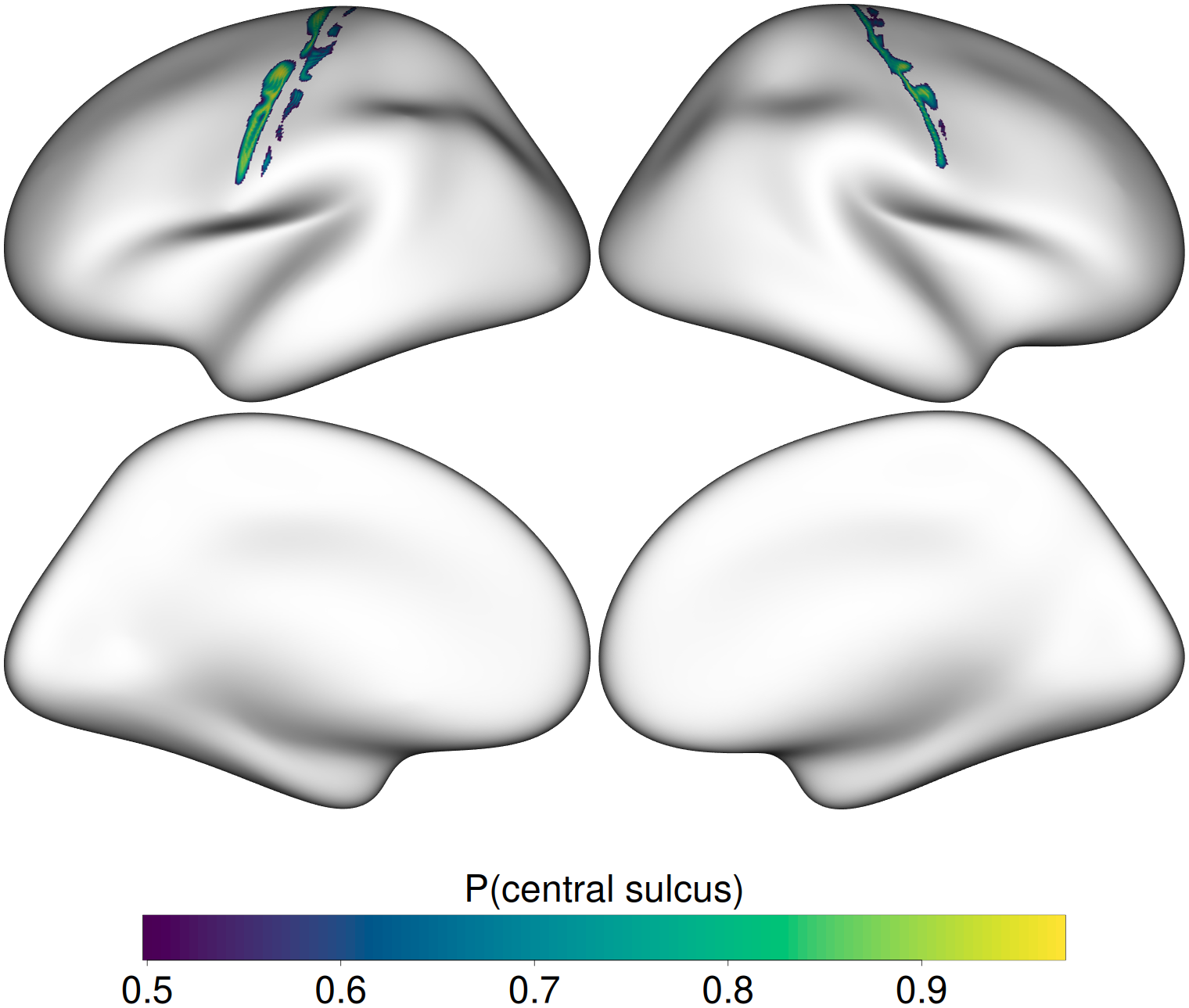
The probability mass hugs the central sulcus on both hemispheres, exactly where it should be — and the automated validation confirms it quantitatively.

Anatomical validation

01_mni_volumetric/run_mni_validation.R finds the peak-probability vertex in each hemisphere and looks up its Desikan–Killiany label on fsaverage. The peak must be precentral, postcentral, or paracentral (the gyri that flank the central sulcus). Current output:

  lh: peak P(central sulcus)=0.972 at vertex 854   -> DK label 'precentral'  [PASS]
  rh: peak P(central sulcus)=0.939 at vertex 19673 -> DK label 'precentral'  [PASS]
Workflow A validation PASSED.

The script exits with status 0 on success and 1 on failure, so it can gate continuous integration later.

Rscript run_mni_validation.R